How Qlik Predict Learns Numbers
- Igor Alcantara
- Aug 25, 2025
- 14 min read

Updated: Oct 13, 2025

Author: Igor Alcantara
When someone says “regression,” your brain might first jump to childhood flashbacks of questionable fashion choices or to the time you fell back into eating instant noodles for dinner three nights in a row. Or maybe regression is the haircut I used in the 1990's when I was the singer and lead guitar player in a rock band (see below). But in the world of data science, regression is about moving forward using past data to predict future values.

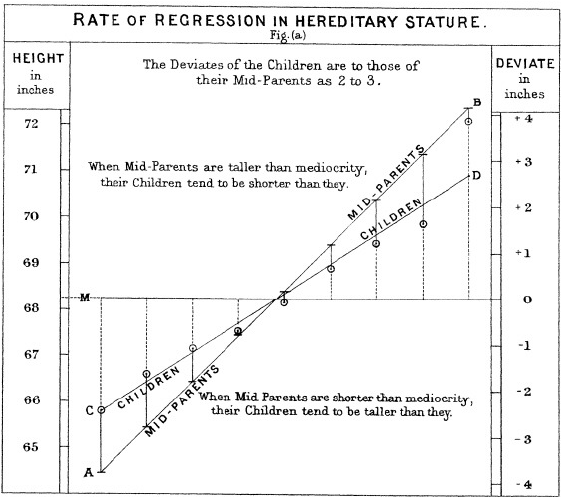
But why Regression is called regression? Great question! The short version is a bit of Victorian history. Francis Galton, one of the founding fathers of modern statistics, studied how traits run in families, especially height. He found that very tall parents tend to have less tall children, a little closer to the population average. Very short parents show the mirror image. He called this effect “regression toward mediocrity” where mediocrity simply meant the mean (average). In his 1886 paper he fit a straight line to predict children’s height from parents’ height, and the slope was less than one, which captures that pull toward the mean. The technique took its name from the phenomenon.
This article is about that. How can we predict numbers and use this to better understand our business? We are about to start another one in our "the Theory behind Qlik Predict" series. For the other articles in this series, please refer to the following list:
What is Regression?
At its simplest, regression is about finding the relationship between variables. Imagine you run a coffee shop. You might notice that your daily sales tend to go up when it’s cold outside and drop when it’s hot. You could plot temperature against coffee sales and see a pattern. Regression is the math that quantifies that pattern so you can make predictions:
If tomorrow is forecast to be 10°C cooler, how much more coffee might I sell?
Regression takes your independent variables (also called features or predictors, like temperature, day of week, or special promotions) and uses them to estimate your dependent variable (target, like number of coffees sold). In a nutshell, you input an X (independent variable) and outputs a prediction Y (dependent variable).
Sounds interesting, right? How do you do it? What is the process? Do I need to write a series of if statements and write down the business logic? No! That would be insane. There are so many possible scenarios, so many different variables, that would be impossible to write it all in a piece of code. We do not do that. Instead, we use science greatest shortcut: math!
In summary, we do not inform all of the business logic to a code in order to make predictions, we use math to build a formula where, providing the input, it will calculate the most probable output. It does not do this by an act of magic. It is a methodology that uses information from the past, data where we already know the output (y) and learns how each piece of the input (x) interact to produce a given result. There is a recipe for this challenge. A recipe to perform a task in computer science is called an Algorithm (from the 9th century Persian scholar Muḥammad al-Khwārizmī, or al-Goritimi in medieval Latim).
Actually, not one algorithm, but multiple, dozens of them, like dozens of different roads to achieve your destination. Many algorithms and new ones are crafted every year. Which one is the best for my problem? It is hard to know before trying out a few. Different algorithms see data in different ways. Some are happy with straight line structure, others hunt for interactions and thresholds, some handle many categories with ease, and others thrive on millions of rows. The "No Free Lunch" theorem reminds us that no single method wins on every dataset, so the only honest way to choose is to train a bunch of models and compare their errors to select the one with the best performance.
Regression in Qlik: Six Algorithms, One Goal
Doing that programmatically in Python or R means building pipelines for cleaning, encoding, scaling, tuning, cross validation, tracking, and reporting, which is slow and fragile work. Qlik Predict turns that grind into a guided evaluation, runs the comparison for you, and surfaces clear metrics and explanations so teams can reach a trustworthy model faster, which is real democratization of machine learning.
Even so, we know that at the end of the day, the best option will be in between a handful of algorithms. That's why Qlik Predict stick with the most logical six. Other tools like Data Robot have a few dozens of them, including the very expensive Neural Networks. However, you don't need the fancy ones, you need the ones that work. Imagine your mission is to kill a bug who entered your bedroom. What are your options for tools? Not many, a sandal, an old newspaper, maybe a bug spray and that's pretty much it. Could you use a flame torch, a AK-47 or your mother-in-law? Technically yes, but that will be a very expensive and traumatic endeavor.
In Qlik Predict, regression is one of the three pillars of modeling (alongside classification and the soon-to-come time series forecasting). It’s the go-to when you need to predict a continuous numerical outcome: sales, prices, demand, revenue, temperature, time spent on a task, how much to spend on a gift so your spouse will forgive the fact you did not remember your anniversary, you name it.
Qlik Predict’s ML approach means you don’t have to select or tune algorithms yourself. It tests multiple models, compares their performance, and gives you the champion. All of that with no line of code written (sorry Python developers, we do not need you for this). But knowing what’s under the hood helps you understand why the model works, what its strengths are, and where its limitations might lie.
So, let’s explore regression from the ground up and we meet the six algorithms Qlik Predict uses. I will first explain each algorithm the best way I can and later, I will summarize what we learned with a bullet point list and a simple "when to use" table. You don't want to understand the algorithms in detail and just need the "short version? Click here to jump to the summary section.
1 - Linear Regression

This one is the honest accountant of the group. It draws the straightest possible line through your cloud of dots and says, “Here is the deal. For every extra unit of X, Y usually goes up or down this much.” It is fast, clear, and great when the world behaves and when relationships are simple and linear. If the pattern really is a straight line, it nails it. If the pattern is a roller coaster, it shrugs and gives you a straight ramp. Outliers can go off track like a toddler with a shopping cart, so a quick clean up helps.
It can struggle when there are strong curves, threshold effects, or a few extreme outliers pulling the line where it should not go. Residual plots should look like random noise; if they fan out or bend, the model is hinting that it wants a different shape. Honestly, I have never used a Linear Regression in a real business case, I prefer the gradient methods. The world is not simple, Dorothy, is messy and wild. So, don't worry much about this algorithm.
2 - Random Forest Regression

Before talking about the Forest, let's understand the Tree. Think of a decision tree as a smart flowchart. It asks simple yes or no questions in sequence until it lands on a leaf, then it gives you a number. For house price it might ask, Is the size above 1,500 square feet? If yes it asks another question. If not it goes a different way. Each leaf stores the average price of the training rows that ended there, so the prediction is the leaf’s average. Trees are great at rules like thresholds and interactions. They are also a little moody. One odd sample can change a split and the whole path shifts.
How about the Forest? Instead of trusting one moody tree, train a whole crowd of them on different shuffles of the data and different subsets of the columns. Each tree makes its own guess. You average the guesses to get the final number. The randomness makes the trees disagree in useful ways and the averaging cancels their quirks. Forests handle twists and turns in the data, work well with a mix of numbers and categories, and usually give steady results without much fuss. They are not great at predicting far outside the range they have seen, since leaves answer with local averages, and they explain themselves with feature importance rather than tidy equations.
3 - XGBoost Regression

The picture shows XGBoost as a stack of small trees whose outputs are added. Each tree makes a few simple feature splits and lands in a leaf with a tiny number that acts like a correction to the current guess. Trees are trained one after another and their leaf values are summed, with each tree’s effect shrunk a bit by the learning rate, so the final prediction is a weighted sum of many small fixes. The plus sign is a reminder that nothing gets replaced, everything is added, which is how the model keeps improving step after step.
This is my sweetheart favorite one. Imagine a coach who replays the tape after every play and fixes the exact mistake that just happened. Or maybe a groundhog day moment when the same sample is relived multiple times. That is XGBoost. It builds a small tree, checks what it got wrong, builds another small tree to fix that, and keeps going until the misses are tiny. The careful step size keeps it from overreacting. The result is often top accuracy on structured data. It does need guardrails like early stopping, or it may start memorizing quirks that are not real signal. When you want every last point of performance, this is your clutch player.
XGBoost stands for eXtreme Gradient Boosting. The X means eXtreme, a nod to the focus on speed and accuracy through clever engineering and regularization. The G means Gradient, the math term for the direction that most quickly reduces the model’s error. The Boost is boosting, a method that adds many small trees in sequence so each new tree fixes what the previous ones missed. Put together you get a fast, accurate model that keeps correcting itself until the misses are small.
Still curious? Let me go a little deeper. A gradient is the direction that most quickly lowers the model’s error. Imagine hiking in fog toward a valley. You feel which way the ground tilts the most downward and step that way. Keep repeating and you reach the bottom fast. During training, a model does the same with error. It senses the direction that drops error fastest and nudges its parameters that way.
Boosting is teamwork for small models; you train a tiny tree, check what it missed, train the next tree to fix those misses, and keep stacking these small fixes until the group gives a strong prediction. For example, predicting house price starts simple. The first tiny tree guesses one average price for everyone, say 320,000, which leaves big errors. The next tiny tree learns a size rule and fixes large homes being under predicted. Another learns a neighborhood premium. Another spots the effect of recent renovation. Each new tree fixes what the last one missed and the team prediction gets sharp.
4 - SGD Regression

SGD Regression is a linear model trained with stochastic gradient descent. It is a linear model that learns in small bites. Think of a biker learning a new city one block at a time. The model looks at a few rows, tweaks the line a little, shuffles to a few new rows, tweaks again, and keeps repeating until the errors settle down. That is what stochastic means here. It samples small random chunks rather than chewing the entire table at once.
The descent part is the direction of fastest error drop. Each tiny step moves the coefficients where the error falls the quickest. A learning rate controls the size of the step. Too large and the model runs quick but it does not fine tuned too well, it looses accuracy. Too small and it runs forever. Regularization can be added to keep coefficients sensible, which helps when many columns tell a similar story.
This approach is light on memory and fast in practice. It shines on very large tables, on streaming data, and on very wide and sparse features like text counts. It prefers features that live on similar scales. If one column is in dollars and another is in yards, the model will walk unevenly unless you standardize. You need to standardize basically because you don't want one a column (feature) to be considered more important just because it has larger numbers. Qlik Predict handles that during preprocessing so you do not have to.
Use SGD when you want a strong baseline quickly or when the dataset is simply too large for heavier methods. It may not be the final champion every time, yet it often gets you close with a fraction of the effort.
5 - LightGBM Regression

LightGBM is the fast cashier of boosted trees or a very smart store manager. It turns continuous numbers into tidy buckets, which lets it test split points very quickly. When I say split think of some kind of decision trees. Imagine a store that sorts items into labeled bins before opening. Finding what you need takes seconds instead of minutes.
Training puts effort where it matters most. The model grows trees leaf wise, which means it keeps expanding the branch that still has the biggest mistakes. Easy parts of the data get a light touch. Hard parts get more attention until the errors shrink.
LightGBM uses a few smart shortcuts. It focuses on examples that teach the most and skims the easy ones, so training speeds up without losing accuracy. It can also bundle features that rarely appear together into one compact group, which cuts the work while keeping the signal you care about.
The image above presents LightGBM regression as an ensemble of decision trees arranged sequentially; each tree uses leaf-wise splits, which is a distinctive feature of LightGBM that lowers error by focusing on the most impactful splits; resulting in deeper, more complex branches. As each tree learns from prior mistakes, its predicted values are aggregated, gradually refining the overall model’s accuracy. The image highlights how combining multiple trees with leaf-wise splitting produces a powerful additive structure, which explains LightGBM’s efficiency in handling large, high-dimensional regression tasks.
Speed is the headline and accuracy comes along for the ride, especially on large, busy datasets. On very small datasets it can get a bit too enthusiastic and start fitting noise, or overfitting. Simple guardrails help. Set a reasonable maximum depth. Ask for a bigger minimum number of rows in each leaf. Turn on early stopping and let a real validation fold tell the model when to quit.
If you want the boosted tree feel of XGBoost with shorter training time, LightGBM is a strong pick. It moves fast, focuses on the right places, and usually gives you a sharp answer without a long wait.
6 - CatBoost Regression

CatBoost is the model that speaks fluent category. Product, city, plan, customer, all come in as plain labels and it handles them without a circus of dummy columns or guessy numeric codes. During training it builds running statistics for each label using only earlier rows, so it keeps real signal and never peeks at the answer. The trees it grows are small and tidy, then stacked so each one trims a bit more error. Scoring stays quick, accuracy stays steady, and setup is pleasantly light.
Business tables with lots of labels and thousands of unique values are its home turf. Many data scientists now call CatBoost a new favorite because the defaults are strong, results land well on real data, and SHAP explanations plug in smoothly when someone asks “why did this number move.”
Cat stands for categorical and Boost is short for boosting, the trick of stacking many small trees so each one fixes a bit of the remaining error. The name tells you two things at once. It is a boosted model and it is built to handle categories without a lot of prep.
So, if it is a Categorical Boosting, why do we use it for Regression? Well, we use it for both. Transforming a numerical problem into a categorical one usually makes it simpler to solve. Regression means the thing you predict is a number. It does not say anything about the types of inputs you feed the model. Categories often explain numbers very well. Neighborhood helps explain house price. Subscription plan helps explain monthly revenue. Product family helps explain return rate. CatBoost turns those labels into clean numeric signals during training and uses them to predict a continuous target. That is why a model designed for categorical inputs can be excellent at regression.
CatBoost regression works in small, careful steps. Start with the overall average of the target. Grow a tiny tree that asks a few yes or no questions such as Area ≥ 500 or Has AC, then add the leaf’s value you land on to that baseline. Check what is still wrong, the leftover error, and train another tiny tree that tries to correct it using other splits like Bedrooms and Bathrooms. Keep repeating this add a small correction, check the leftover error routine, with each tree’s effect scaled by a learning rate so no single step dominates. The final prediction is simply the baseline plus the sum of all those small corrections.
Let's summarize
In a few words, this is what each algorithm is and when they are mostly useful.
1. Linear Regression: The Straight Shooter
Fits a straight line (or plane) through your data, minimizing the sum of squared errors.
Strengths:
Simple and interpretable.
Fast to train and use.
Easy to explain to non-technical stakeholders.
Weaknesses:
Assumes relationships are linear.
Sensitive to outliers.
Struggles with complex, non-linear data patterns.
When Qlik Might Use It: When your data shows a clear, straight-line trend and interpretability is a priority.
2. Random Forest Regression: The Crowd Voter
Builds many decision trees, each on a random subset of the data and features. Predictions are averaged.
Strengths:
Captures non-linear relationships easily.
Handles categorical and numerical features.
Resistant to overfitting.
Weaknesses:
Slower with large datasets.
Less interpretable (you can’t just “see” the model).
When Qlik Might Use It: When the data is messy, relationships are complex, and stability is more important than transparency.
3. XGBoost Regression: The Overachiever
Gradient boosting on steroids; builds trees sequentially, with each tree correcting the errors of the previous one.
Strengths:
Often best-in-class accuracy.
Handles missing values gracefully.
Works well on structured/tabular data.
Weaknesses:
Can overfit if not tuned.
More computationally expensive.
When Qlik Might Use It: When the dataset is moderately large and you want maximum predictive performance.
4. SGD Regression: The Speed Demon
Uses Stochastic Gradient Descent to update coefficients in small, random batches instead of solving in one shot.
Strengths:
Extremely fast and memory-efficient.
Scales to millions of records.
Weaknesses:
Requires careful learning rate tuning.
Can be unstable if features aren’t scaled.
When Qlik Might Use It: When speed is essential and you have huge datasets where other algorithms would choke.
5. LightGBM Regression: The Tactical Player
Concept: Leaf-wise tree growth rather than level-wise, focusing on reducing the largest errors first.
Strengths:
Blazing fast training.
Efficient with large datasets.
Handles categorical features natively.
Weaknesses:
Can overfit small datasets.
More complex to explain.
When Qlik Might Use It: When the dataset is large and complex, and you need both speed and accuracy.
6. CatBoost Regression : The Categorical Whisperer
Gradient boosting that internally encodes categorical variables, avoiding manual preprocessing.
Strengths:
Great with lots of categorical features.
Less need for feature engineering.
Robust default settings.
Weaknesses:
Slower training on very large datasets.
Less transparent decision-making process.
When Qlik Might Use It: When your dataset has many categorical variables that would otherwise require heavy preprocessing.
Scenario | Likely Champion |
Simple, linear patterns | Linear Regression |
Complex non-linear data | Random Forest / XGBoost |
Large dataset, speed is key | SGD / LightGBM |
Many categorical features | CatBoost |
Accuracy above all else | XGBoost / LightGBM |
The Final Word
Regression in Qlik Predict is not “linear regression in a fancy UI.” It is a real toolbox stocked with battle tested methods, each one trained, scored, and compared so the best model steps forward. You get numbers you can trust, explanations you can defend, and the freedom to focus on the decision instead of babysitting code.
Curiosity about the algorithms is not optional, it is power. When you know what is inside the box, you read SHAP with confidence, spot drift before it bites, and pick the right error metric for the way your business actually loses money. That turns a model from a neat chart into a lever that moves the plan.
Ship models, watch them, retrain them, keep learning. Qlik Predict handles the heavy lifting and keeps the tournament fair. You bring the questions that matter and the courage to act on the answers. That is how regression stops being a classroom word and becomes a competitive edge.


Comments